Probabilities with Perfect Information
Presidential elections over the past 40 years
You can trust state polling, but should ignore the election forecast probabilities.
TL;DR
Only landslide elections over the past 40 years had a probability over 90% for the favored candidate. Close elections between two candidates, just like a coin toss, are within a few points of a 50% probability for both candidates. The most popular election forecaster overestimates the probability for the victor by 20%.
What I will cover in this post
- Using actual state level results instead of polling data
- Every election results compared to the probability starting from 1980
- Examining the three missed states of 2016 election forecasts
Elections are the only polls that matter
The baseline for forecasters to create state probabilities is polling data from a variety of sources. This is a two-step process. The first step is to come up with the percentage of votes each candidate will receive on election day. The second is to then determine the probability a candidate will have the largest proportion of votes. We can consider the final results of a state as perfect data. The results are pefect because we know exactly how every voter who chose to vote cast their ballots. There is no margin of error to consider.
Polling surveys include a margin of error because they are sampling the population of likely voters. In other words, they are creating estimates of the final results. Since it is not possible to determine who exactly will vote, pollsters use the term likely voters, the subset of registered voters that are most likely to cast ballots for election day.
Even though we have perfect state data, we will add in a margin of error for each state so we can create probabilities in the same manner as election forecasters. The simulations conducted use the framework written by Drew Lizner. You can read more about it here. For his simple model, Linzer assumed a 5% degree of uncertainty in state polls and 3% in national polls. The 10,000 simulations I will run for each election will do the same. This means that a state poll can be plus or minus 5 points. In addition, the national polls will represent a national trend shifting all state polls in each simulation plus or minus 3 points.
Every Presidential Election since 1980
Simulations were run in Jupyter Notebook. If you would like to see exactly how the simulations were ran in python, you can find a copy of the notebook at the link above.
1980: Reagan vs. Carter
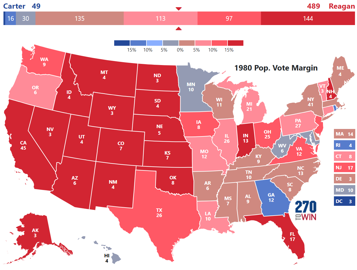
The 1980 election is a classic example of a landslide victory. The simulation generated probabilities that reflect the same.

This brings us to our first finding. Only landslides should have above a 90% probability. Excessively high probabilities was one of the most misleading elements of election forecasts in 2016.
1984: Reagan vs. Mondale
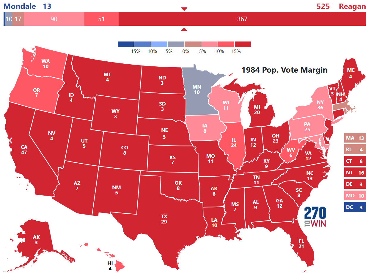
The 1984 election is the largest landslide victory over the past 40 years. As expected, the simulation generated the highest probability for a victory.

Even though the simulation injects uncertainty at the state and national level, we have our first and only probability with near certainty of the outcome.
1988: Bush vs. Dukakis
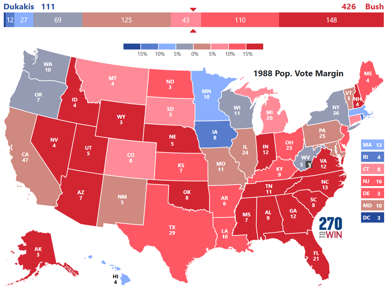
The 1988 election was the last election we will see with a probability of victory for a candidate above 90%.

This election sets the bar for the minimum we should consider when a candidate is claimed to have a 90% probability of winning. George H.W. Bush averaged 388 electoral college votes, 118 above the necessary 270 votes to win.
1992: Clinton vs. Bush
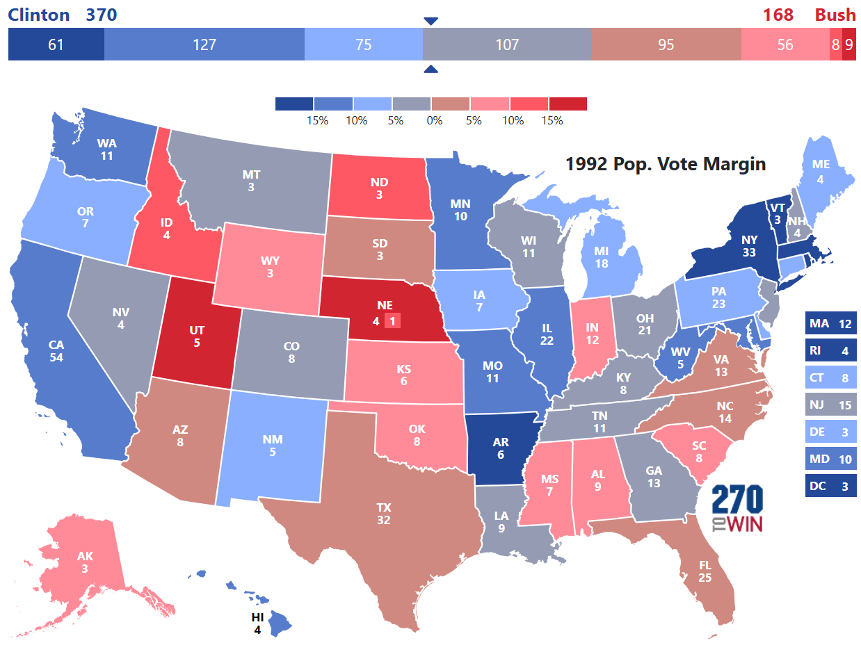
Qualitative assessments from political scientists will discuss the third party effect and cite the presidential campaign of H. Ross Perot. The simulation did not output results that would support or refute such analysis.

The 1992 election gives us our first change of power in the White House, but still yielded a high probability for the victor at 82.4%.
1996: Clinton vs. Dole
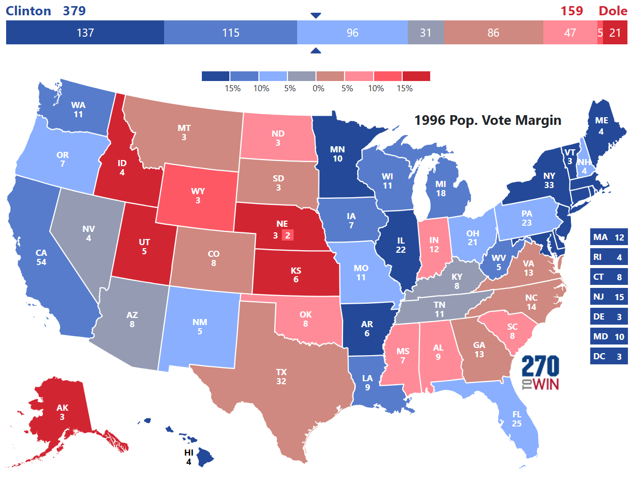
The 1996 election will be the second election Clinton would win and also the lowest turnout for an election since 1924.

Although the electoral college votes increased by 9, we see Clinton having a probability for victory of 88.5%. The probability for a Clinton win is very close to what George H.W. Bush averaged in the 1988 simulations that gave him a 92% chance of victory.
2000: Bush vs. Gore
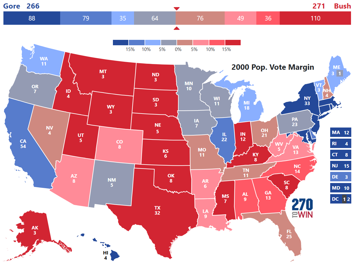
Famous for the "hanging chad" from the Florida recount, the 2000 presidential election simulation correctly provided probabilities reflecting a close election. This simulation provided us with our second finding; close elections should have probabilities close to 50/50 odds.

Three points to highlight from this election. George W. Bush averaged 278 in the simulations which is above the 271 final electoral college result indicating that his most frequent simulated paths to victory did not come down to Florida. In fact, his most common result was 264, which is losing the election. Being on both sides of 270 electoral college votes in terms of average and most common outcome validates his simulated probability of victory at 54.3%
2004: Bush vs. Kerry
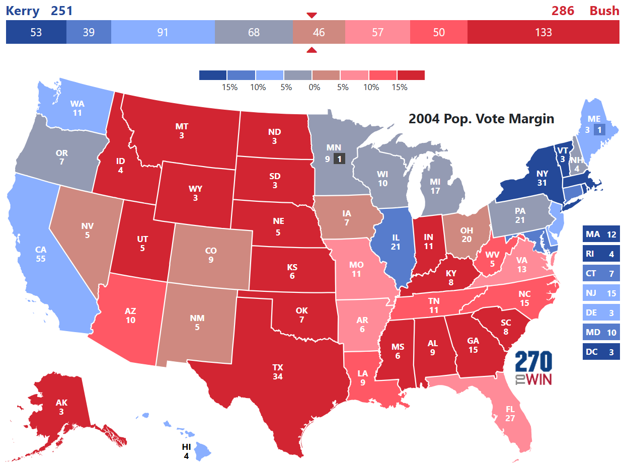
The second election of the modern "Red State, Blue State" era gave us another election decided by a single state; Ohio. The difference being this election did not require a decision by the Supreme Court and the probabilities had a favorite.

We see the electoral college range of simulated results shift beyond the margin of victory for Bush giving him a 67.2% probability for victory. Although it was a one state determination yet again, he had a number of state combination paths to win in the simulations.
2008: Obama vs. McCain
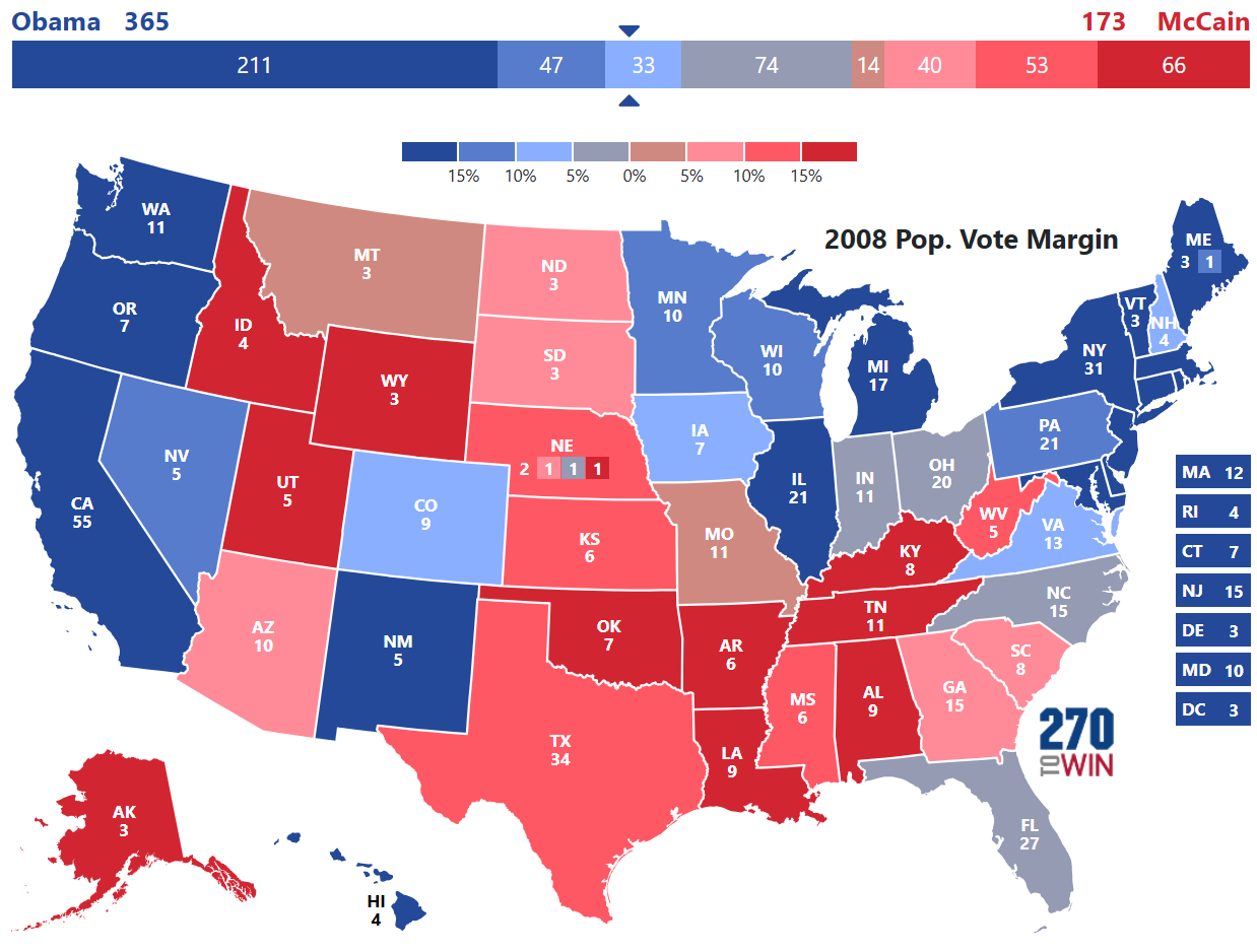
The historic election gave us one of the highest probabilities for victory since the 1996 Clinton win.

Simulations generated a 86.1% probability of victory with the final result being beyond the most common simulation result and simulation average. This election also brought forecasters into the spotlight of national media attention.
2012: Obama vs. Romney
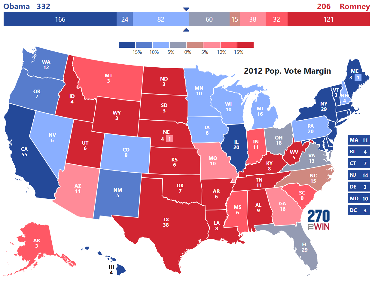
The year prior, the movie Moneyball was released and won a number of awards and nominations. The 2012 election was the first where election forecasters made almost as many headlines as the candidates. Nate Silver became the subject of a number of memes post-election. Even though he correctly forecasted 50 out of 50 states, his probability for victory was higher than our simulation.

Silver used weighted state polling data and simulations to come up with his probability, but it is far away from the probability generated with perfect data.

With perfect information and intentionally injecting uncertainty into the simulation, it did not produce a probability of victory as high as Silver. The 90.9% probability is nearly 20% higher than the simulation results of 71.2%.
2016: Trump vs. Clinton
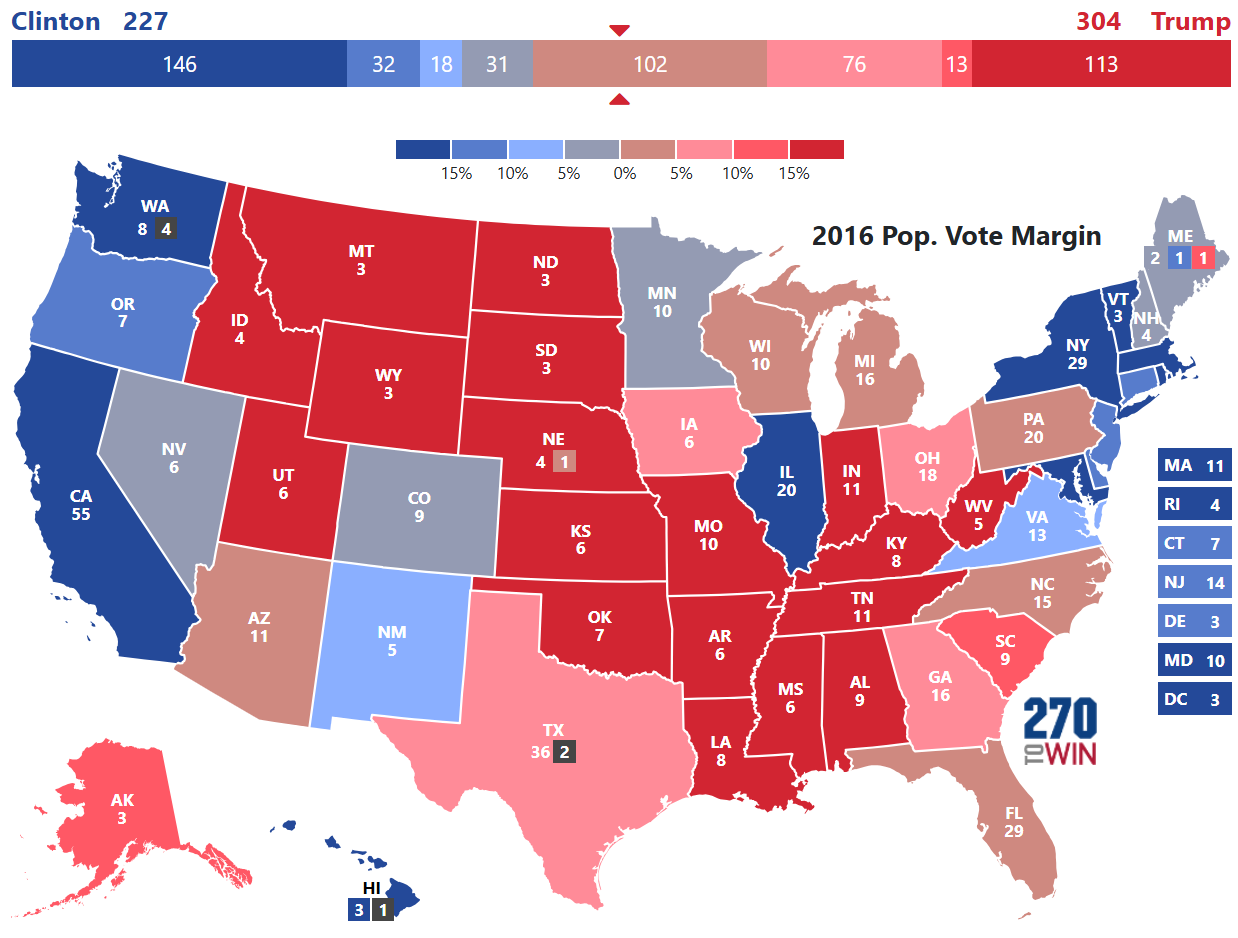
Election forecasts and polling have been a topic of discussion in presidential elections because of this race, as it shattered confidence in polling and forecasts for many.

Post-election, some credited Silver with giving Trump the highest probability for victory as other forecasts had a probability for Clinton at 90% or higher.

For a second time, the probability published by Silver is 20% off of what was generated from perfect information with uncertainty injected into the simulation. Just like Bush in 2000, we see Trump having his most common simulated outcome and simulation average straddling the line of victory. What is interesting to note, is that unlike Bush in 2000, his most common simulation outcome is a loss while his simulation average is a win. Even with perfect information on the outcome, Trump still generates a probability of victory at 47.5%. This also shows that Clinton was marginally favorited to win, but by a much smaller margin than published by forecasters, including less aggressive ones like Silver.
The Three Missed States
As we have seen, injecting uncertainty into a simulation with perfect data on the outcome gives us a more realistic probability on the actual outcome. We have also seen that the leading forecaster has been consistently off in probabilities by nearly 20% when compared to the probabilities generated by perfect data. Before drawing any conclusions, we will examine the three states missed my nearly all forecasters in 2016.
Pennsylvania

Silver gave PA to Clinton over 3 out of 4 times, carrying 20 electoral college votes.

Pollsters and qualitative experts labeled PA as a toss up state. The simulation generated probabilities inline with such analysis, slightly above 50/50.
Michigan

Silver gave MI to Clinton over 8 out of 10 times, carrying 16 electoral college votes.

Another state pollsters and qualitative experts labeled a toss up state. The simulation generated probabilities were again inline with such analysis, slightly above 50/50.
Wisconsin

Silver gave WI to Clinton nearly 9 out of 10 times, carrying 10 electoral college votes.

While pollsters did not label this a toss up, no polling averages had Clinton with a majority; meaning over half of likely voters. As we have seen above, if it is not a landslide, it should not carry a chance of victory close to 90%.
Summary
With probabilities for these states so high, a simulation would award 46 electoral college votes to Clinton about 70% of the time resulting in a simulation victory. This is aligned with Silver's probabilty of a Clinton victory.
Conclusion
We have boundaries for probabilities based on the presidential elections over the past 40 years.
- If the probability for victory is above 90%, then the electoral college estimate should be above 400.
- If the probability for victory is above 80%, then the electoral college estimate should be above 330.
- If the probability for victory is above 70%, then the electoral college estimate should be above 300.
- States that are toss ups should be considered 50/50 states.
Any forecaster not transparent with how they derive their probabilities has to be met with some healthy skepticism that they were lucky before or putting their thumb on the scale. If forecasts have probabilities that do not align with historically generated probabilities from perfect data with uncertainty injected into the simulations, they are inaccurate at best and clickbait at worst.
It is best to focus on the polling coming out of battleground states, rather than complex models with obfuscated methods of generating probabilities for potential winners.
You can find my election updates at the link below:
Understanding the 2020 Presidential Election Polls