Understanding the 2020 Presidential Election Polls

Final Update: November 3, 2020
For Election Night
Safe States and Swing States: How to track the 2020 Presidential election November 2, 2020
Why is 2020 Different from 2016?
Simple answer is that there is a smaller percentage of undecided and 3rd party voters. Here is a table comparing polling averages from 2016 and 2020 in potential swing states.
| State | Biden (D) | Trump (R) | Undecided & 3rd Party 2020 | Clinton (D) | Trump (R) | Undecided & 3rd Party 2016 | |
|---|---|---|---|---|---|---|---|
| 0 | North Carolina | 48.8 | 46.5 | 4.7 | 45.5 | 46.5 | 8 |
| 1 | New Hampshire | 53.4 | 42.4 | 4.2 | 43.3 | 42.7 | 14 |
| 2 | Texas | 45.5 | 49.5 | 5 | 38 | 50 | 12 |
| 4 | Florida | 48.9 | 46.8 | 4.3 | 46.4 | 46.6 | 7 |
| 5 | Arizona | 49.5 | 46.3 | 4.2 | 42.3 | 46.3 | 11.4 |
| 6 | Wisconsin | 49.3 | 44.7 | 6 | 46.8 | 40.3 | 12.9 |
| 7 | Ohio | 46.2 | 46.8 | 7 | 42.3 | 45.8 | 11.9 |
| 8 | Pennsylvania | 49.5 | 44.6 | 5.9 | 46.2 | 44.3 | 9.5 |
| 12 | Michigan | 50.4 | 42.6 | 7 | 45.4 | 42 | 12.6 |
| 13 | Iowa | 47.2 | 46.4 | 6.4 | 41.3 | 44.3 | 14.4 |
| 14 | Virginia | 51.7 | 40.3 | 8 | 47.3 | 42.3 | 10.4 |
| 15 | Nevada | 49 | 43.8 | 7.2 | 45 | 45.8 | 9.2 |
| 16 | Georgia | 47.5 | 46.3 | 6.2 | 44.4 | 49.2 | 6.4 |
TL;DR Scenarios
States with a weighted polling average of 50% or higher
| Candidate | Strong | Likely | Total |
|---|---|---|---|
| Biden | 173 | 45 | 218 |
| Trump | 67 | 44 | 111 |
If ALL undecided voters in every state vote for Trump
| Candidate | Strong | Likely | Total |
|---|---|---|---|
| Biden | 181 | 37 | 218 |
| Trump | 295 | 25 | 320 |
Randomized distribution of undecided voters in every state
| Candidate | Strong | Likely | Total |
|---|---|---|---|
| Biden | 227 | 107 | 334 |
| Trump | 111 | 93 | 204 |
NEW
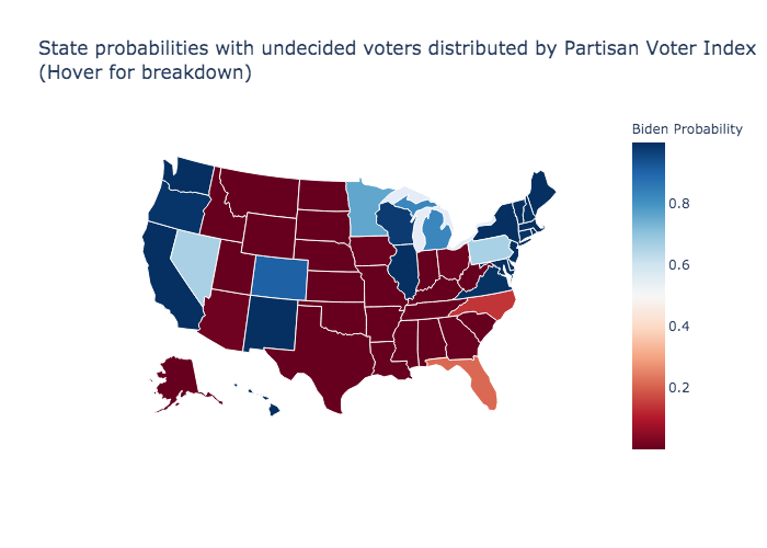
Undecided voters distributed by Partisan Voter Index
| Candidate | Strong | Likely | Total |
|---|---|---|---|
| Biden | 227 | 52 | 279 |
| Trump | 215 | 44 | 259 |
Update
I added a fourth scenario to demonstrate how undecided voters can change the outcome of the election. This one uses the Cook Political Report’s Partisan Voter Index to weight how to distribute undecided voters. Keep in mind that an electoral college tally of 270 and above is a win so when a scenario has a winner, that total will be in bold.
Strong and Likely States
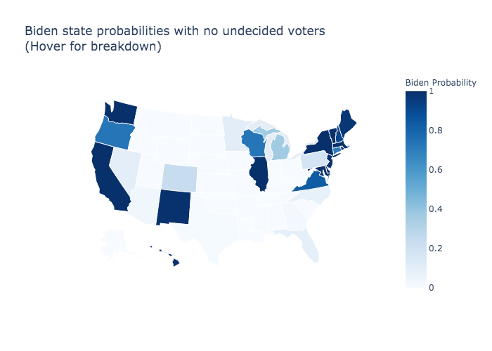
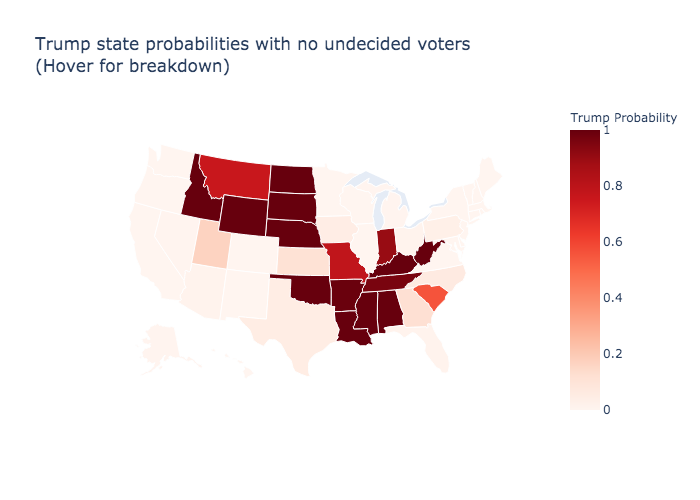
In the two graphics below, we have states that are considered strong or likely states for the two candidates. The probability is based upon the weighted average polling for each state and if a candidate can win the state without the support of any undecided voters. Safe states without polling as designated by the Cook Political Report are assigned a probabilty of 1 for the favored candidate and 0 for the opponent.
Biden
Biden Solid States 173
Biden Likely States 45
Biden Solid + Likely States 218
Link to Interactive graphic
Biden Solid and Likely States
Trump
Trump Solid States 67
Trump Likely States 44
Trump Solid + Likely States 111
Link to Interactive graphic
Trump Solid and Likely States
States where undecided voters are most likely to determine the outcome
The table below can be considered the “path to victory” states as both campaigns will pursue several combinations of these states to pass 270 electoral college votes.
| State | ec | cook | PVI | Biden_avg | Trump_avg | undecideds | |
|---|---|---|---|---|---|---|---|
| 1 | arizona | 11 | Lean Dem | R+5 | 47.4 | 46.8 | 5.8 |
| 2 | colorado | 9 | Likely Dem | D+1 | 49 | 39.3 | 11.7 |
| 3 | florida | 29 | Toss Up | R+2 | 48.1 | 46.7 | 5.2 |
| 4 | georgia | 16 | Toss Up | R+5 | 47.1 | 48.3 | 4.5 |
| 5 | iowa | 6 | Toss Up | R+3 | 45.8 | 47.5 | 6.7 |
| 6 | michigan | 16 | Lean Dem | D+1 | 49.5 | 46.2 | 4.3 |
| 7 | minnesota | 10 | Lean Dem | D+1 | 48.2 | 44.1 | 7.7 |
| 8 | nevada | 6 | Lean Dem | D+1 | 48.1 | 46.1 | 5.8 |
| 9 | north carolina | 15 | Toss Up | R+3 | 48 | 47.8 | 4.3 |
| 10 | ohio | 18 | Toss Up | R+3 | 45.6 | 46.7 | 7.6 |
| 11 | pennsylvania | 20 | Lean Dem | EVEN | 48.7 | 47.2 | 4.1 |
| 12 | texas | 38 | Toss Up | R+8 | 46.4 | 47.6 | 6 |
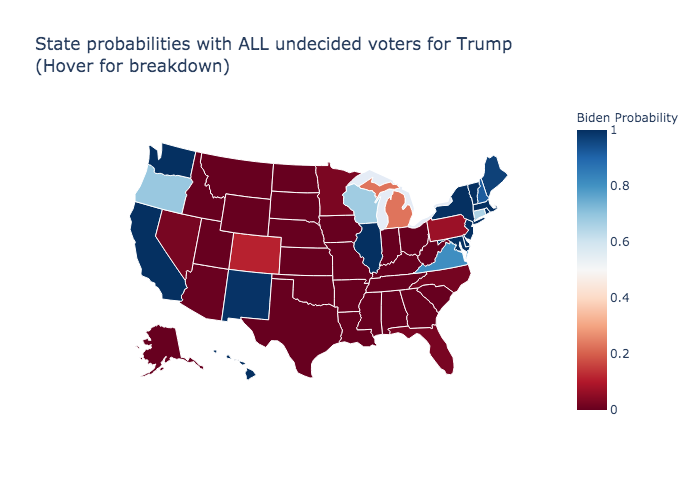
If all undecided voters are shy Trump supporters
The graphic below assumes all undecided voters will vote for Trump. This scenario is the “hidden Trump vote” or “shy Trump supporter” in polling.
Trump Solid States 295
Trump Likely States 25
Trump Solid + Likely States 320
Biden Solid States 181
Biden Likely States 37
Biden Solid + Likely States 218
Link to Interactive graphic
Hidden Trump Vote Scenario
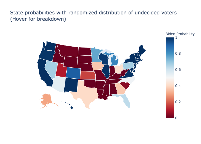
Random distribution of undecided voters
The graphic below randomly distributed undecided voters for each state in 20,000 simulations per state.
Trump Solid States 111
Trump Likely States 93
Trump Solid + Likely States 204
Biden Solid States 227
Biden Likely States 107
Biden Solid + Likely States 334
Link to Interactive graphic
Randomized undecided voters
Partisan Voter Index distribution of undecided voters
The graphic below uses the PVI to determine how to distribute undecided voters for each state in 20,000 simulations per state. This is the equivalent of a Polls Plus model.
Trump Solid States 215
Trump Likely States 44
Trump Solid + Likely States 259
Biden Solid States 227
Biden Likely States 52
Biden Solid + Likely States 279
Link to Interactive graphic
PVI undecided voters
Updated Weighted Polls, Cook Political Report Assessment, and Partisan Voter Index
| State | ec | cook | PVI | Biden_avg | Trump_avg | undecideds | |
|---|---|---|---|---|---|---|---|
| 0 | alabama | 9 | Solid Rep | R+14 | 38.3 | 57.7 | 4 |
| 1 | alaska | 3 | Likely Rep | R+9 | 41.4 | 46.2 | 12.4 |
| 2 | arizona | 11 | Lean Dem | R+5 | 47.4 | 46.8 | 5.8 |
| 3 | arkansas | 6 | Solid Rep | R+15 | 39.2 | 53.7 | 7.1 |
| 4 | california | 55 | Solid Dem | D+12 | 61.7 | 30.5 | 7.8 |
| 5 | colorado | 9 | Likely Dem | D+1 | 49 | 39.3 | 11.7 |
| 6 | connecticut | 7 | Solid Dem | D+6 | 50.9 | 33.9 | 15.2 |
| 7 | delaware | 3 | Solid Dem | D+6 | 54.8 | 34.3 | 10.9 |
| 8 | florida | 29 | Toss Up | R+2 | 48.1 | 46.7 | 5.2 |
| 9 | georgia | 16 | Toss Up | R+5 | 47.1 | 48.3 | 4.5 |
| 10 | indiana | 11 | Likely Rep | R+9 | 39.5 | 52 | 8.5 |
| 11 | iowa | 6 | Toss Up | R+3 | 45.8 | 47.5 | 6.7 |
| 12 | kansas | 6 | Likely Rep | R+13 | 40.8 | 48.2 | 11 |
| 13 | kentucky | 8 | Solid Rep | R+15 | 38.6 | 56.4 | 5 |
| 14 | louisiana | 8 | Solid Rep | R+11 | 36.7 | 54.8 | 8.5 |
| 15 | maine | 4 | Likely Dem | D+3 | 52.9 | 39.3 | 7.7 |
| 16 | maryland | 10 | Solid Dem | D+12 | 59.7 | 31.5 | 8.8 |
| 17 | massachusetts | 11 | Solid Dem | D+12 | 63 | 28.6 | 8.4 |
| 18 | michigan | 16 | Lean Dem | D+1 | 49.5 | 46.2 | 4.3 |
| 19 | minnesota | 10 | Lean Dem | D+1 | 48.2 | 44.1 | 7.7 |
| 20 | mississippi | 6 | Solid Rep | R+9 | 41 | 56 | 3 |
| 21 | missouri | 10 | Likely Rep | R+9 | 43.8 | 51.2 | 4.9 |
| 22 | montana | 3 | Likely Rep | R+11 | 43.5 | 51.1 | 5.4 |
| 23 | nevada | 6 | Lean Dem | D+1 | 48.1 | 46.1 | 5.8 |
| 24 | new hampshire | 4 | Lean Dem | EVEN | 52.2 | 42.8 | 5 |
| 25 | new jersey | 14 | Solid Dem | D+7 | 57.3 | 37 | 5.7 |
| 26 | new mexico | 5 | Solid Dem | D+3 | 53.8 | 40.8 | 5.4 |
| 27 | new york | 29 | Solid Dem | D+11 | 59.2 | 31.8 | 9.1 |
| 28 | north carolina | 15 | Toss Up | R+3 | 48 | 47.8 | 4.3 |
| 29 | ohio | 18 | Toss Up | R+3 | 45.6 | 46.7 | 7.6 |
| 30 | oregon | 7 | Solid Dem | D+5 | 51 | 39 | 10 |
| 31 | pennsylvania | 20 | Lean Dem | EVEN | 48.7 | 47.2 | 4.1 |
| 32 | south carolina | 9 | Likely Rep | R+8 | 44 | 50.3 | 5.7 |
| 33 | tennessee | 11 | Solid Rep | R+14 | 39 | 52.8 | 8.2 |
| 34 | texas | 38 | Toss Up | R+8 | 46.4 | 47.6 | 6 |
| 35 | utah | 6 | Likely Rep | R+20 | 38.4 | 48.6 | 13 |
| 36 | virginia | 13 | Likely Dem | D+1 | 51.5 | 40.5 | 8 |
| 37 | washington | 12 | Solid Dem | D+7 | 57.7 | 31.9 | 10.4 |
| 38 | west virginia | 5 | Solid Rep | R+19 | 38.2 | 56.7 | 5.1 |
| 39 | wisconsin | 10 | Lean Dem | EVEN | 51 | 44 | 5.1 |
| 40 | district of columbia | 3 | Solid Dem | D+43 | nan | nan | nan |
| 41 | hawaii | 4 | Solid Dem | D+18 | nan | nan | nan |
| 42 | idaho | 4 | Solid Rep | R+19 | nan | nan | nan |
| 43 | illinois | 20 | Solid Dem | D+7 | nan | nan | nan |
| 44 | nebraska | 5 | Solid Rep | R+14 | nan | nan | nan |
| 45 | north dakota | 3 | Solid Rep | R+17 | nan | nan | nan |
| 46 | oklahoma | 7 | Solid Rep | R+20 | nan | nan | nan |
| 47 | rhode island | 4 | Solid Dem | D+10 | nan | nan | nan |
| 48 | south dakota | 3 | Solid Rep | R+14 | nan | nan | nan |
| 49 | vermont | 3 | Solid Dem | D+15 | nan | nan | nan |
| 50 | wyoming | 3 | Solid Rep | R+25 | nan | nan | nan |
About this Project
Quite a lot has been written about 2016 election forecasts, polls, and the influence they may have had on voter behavior. A good friend and I were also caught up in the hype around forecast models and which one would be the most accurate. We all know how that turned out.

This project is based off of the lessons learned from the 2016 and 2018 elections. The intent is to inform, not influence, the 2020 presidential election.
What’s different?
Plain and simple, there is not a prediction for the winner. Instead, the intent is to show which states are close, which are not, and what the potential effects undecided voters can have on the outcome. The goal of data journalism is to leave the reader with a better understanding of the complex and that is precisely what we will try to do this time around.
Sources of Polling Data
State polling data will come from RealClearPolitics and not include their state averages for reasons covered in the approach section below. Not all states or districts may have polling available. In these cases, the Cook Political Report’s Electoral Scorecard will be used to complete the picture. The states or districts not having polling data until much later in the campaign are often safe for one candidate while battleground states have polling data updated more frequently.
The Approach
Weighted Averages
Not all polls are of equal quality, but a simple average would treat them that way. Instead, I have two methods to weight the polls; by margin or error and by segment polled, specifically registered voters or likely voters.
A registered voter is someone who is simply registered to vote, while a likely voter is a registered voter who has indicated their intention to vote in the election. Polling firms handle this determination differently, but you can read more about the segments here. Since voter turnout varies from state to state, polls with likely voters are weighted 3 times higher than those with registered voters.
segment_weight = np.where(segment == 'LV',3,1)
Margin of error rises and falls depending on the population size, sample size, and confidence interval of the survey. The larger samples will have a smaller margin of error. Polls are ranked according to margin of error as the second weight used to determine average.
candidate_weighted_average = (polls * MoE ranks * sum(segment_weight)) / sum(MoE ranks * sum(segment_weight))
Safe States, Likely States, and Leaning States
We see these terms on a number of electoral college maps, but it may not be apparent as to why a state has such a label.
One of the major issues with the 2016 election was that strong third party candidate performance led to a number of plurality leads; instances in which no candidate had a majority of 50% or greater. The 2020 election year has a traditional two candidate race, meaning we will see majority victories. This is the foundation for the definitions of the labels below.
Safe State is where a candidate has a majority beyond the margin of error and all undecided votes going to the opponent does not change the outcome.
Likely State is where a candidate has a majority within the margin of error and all undecided votes going to the opponent does not change the outcome.
Leaning State is where a candidate has a majority within the margin of error and all undecided votes going to the opponent can change the outcome.
Toss Up is where no candidate has a majority and a combination of the margin of error and undecided votes divided between candidates changes the outcome.
Margin of Error
We are assuming a 3% margin of error for the weighted averages. why assume a 3% margin of error? The simple answer is that it comes down to sample size based upon population size.
Wyoming is the least populated state with around 600,000 residents. In 2016, there were 258,788 ballots cast for the presidential election. For a population of 250,000 likely voters, a sample size of 782 would have a margin of error of 3.5% and a sample size of 1,527 would have a margin of error of 2.5%.
A population of 100,000,000 has similar sample size requirements, 784 and 1,537 respectively. As you look at polling coming in, you see sample sizes near 1,000 or if you average all the polling sample sizes of a state it is also near 1,000, thus a 3% margin of error for the weighted average of state polls.
You can read more about sample sizes here. The lookup table for required sample sizes is one I have used since grad school.
Monte Carlo Simulation for Probabilities
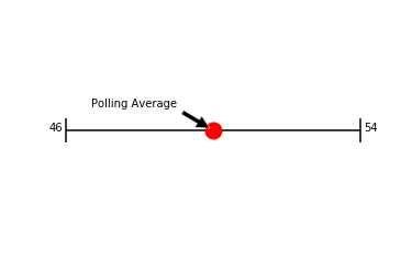
I know upfront I said we are not forecasting a winner and that is still the case. In order to make the state labels easier to understand, we use the weighted averages and 3% margin of error to determine the probability a candidate can win a state without any undecided voter support.
The margin of error gives us a range of what the actual number could be. For example, let’s say a candidate is polling at 50% with a 4% margin of error. That means the actual number would be within this range below.
When we do the same for the competitor, then we can see who may be winning the race. A Safe State for a candidate would look like this
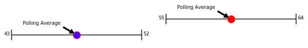
Unfortunately, there are a number of races where the margin of error will overlap. Likely and Leaning States are where we have our first potential area for misinterpretation
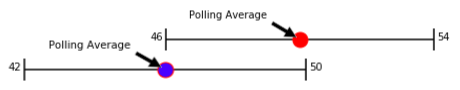
This is why we introduce random error within the range. Using a random number generator for each candidate, we can get a result from a simulation that looks like this below.
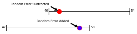
That is one random outcome. What we need to do is figure out how often we can see one candidate ahead of another.
To do a single monte carlo simulation, we would input the respective weighted averages of the candidates and the margin of error and assume normal distribution of the errors.
def moe(x, y, n):
    min_x = x - n
    max_x = x + n
    std_x = (max_x - min_x) / 4
    min_y = y - n
    max_y = y + n
    std_y = (max_y - min_y) / 4
    return round(random.gauss(x, std_x),1), round(random.gauss(y, std_y),1)
Running a simulation one time may lead to an outcome that does not have either candidate with a majority or a sum of votes that does not equal 100% of votes cast.
Undecided Voters
Whenever a round of a simulation does not end up with a total of 100%, we capture that as our undecided voters. The reason this number is important is because undecided voters determine the winner of close races.
def undecided(x,y,n):
    cand1, cand2 = moe(x, y, n)
    u = round((100 - cand1 - cand2),1)
    return round(cand1,1),round(cand2,1),round(u,1)
Now we can run the simulation multiple times in order to generate a probability of how often a candidate can win a majority without any undecided voter support.
def sim(x,y,n,num_sims):
    c1 = []
    c2 = []
    u = []
    c1_wins = 0
    c2_wins = 0
    for i in range(num_sims):
        x1,y1,u1 = undecided(x,y,n)
        c1.append(x1)
        c2.append(y1)
        u.append(u1)
        if x1 > 50:
            c1_wins += 1
        if y1 > 50:
            c2_wins += 1
    return c1_wins/num_sims, round(average(c1),1),c2_wins/num_sims,round(average(c2),1), round(average(u),1)
This gives us a much better perspective on the state of the election race as we can now identify which states are likely to be determined by undecided voters.
Another challenge in interpreting the data remains as the label for Leaning states often gives the false impression that the state will be awarded to that candidate. We saw this scenario play out in the 2016 election as unaccounted for undecided voters tipped several states and the electoral college.
Blog Posts
Safe States and Swing States: How to track the 2020 Presidential election November 2, 2020
Probabilities with Perfect Information: Presidential elections over the past 40 years August 30, 2020
Generals Always Fight the Last War: How the 2020 election is different from 2016 August 16, 2020